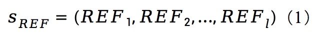
Viral Sequence Feature Extraction Tool
We use paired-end sequencing as an example to explain in detail how to use ViSFE for feature calculation:
1. Input File Preparation
The metadata.txt file containing the sample name
SRR8574911
SRR8574890
SRR8574897
...
The ref_seq.fasta file containing the reference sequence
>ref_seq
ATGGAACACGACCTTGAGAGGGGCCCACCGGGCCCGCGACGGCCCCCTCGAGGACCCCCC
...
The sample.fastq file containing the sequencing data
@DJB775P1:248:D0MDGACXX:7:1202:12362:49613
TGCTTACTCTGCGTTGATACCACTGCTTAGATCGGAAGAGCACACGTCTGAA
+
JJJJJIIJJJJJJHIHHHGHFFFFFFCEEEEEDBD?DDDDDDBDDDABDDCA
...
2. Data quality control and preprocessing
Pre-quality control files:
./data/fastqc/
Clean files:
./data/clean/
Post-quality control files:
./data/fastqc_clean/
Users can check the quality control report and adjust the appropriate parameters for data preprocessing.
3. Sequence alignment and splicing
Reference sequence index files:
./public/reference/
Paired-end sequencing sequence splicing files:
./data/fastqbind/
Sequence alignment
Sequence alignment results of successful splicing: ./result/bwasam/ Sequence alignment results of failed splicing: ./result/unbindsam/
4. Processing comparison results and merging
Extraction and processing of the comparison results
Successful splicing sequence: ./result/cleansample
Failed splicing sequence: ./result/unbindcleansample
Result merging
Merged file: ./result/finaldata/
Read counts for each site: ./result/finaldata/count/
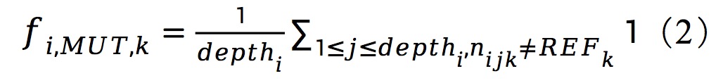
5. Feature calculation
 |
 |
 |
Results files
Feature results: ./feature/data/raw: mutation, count, entropy_nuc, entropy_slide, entropy_group
Number of reads contained in each site: ./feature/data/each
Limiting the sequencing depth
By limiting the sequencing depth, it is easier to build the optimal machine learning model later: ./feature/data/file
Merging all results
./feature/data/sampledata
The final merged feature matrix is shown below:
| Sample | Group | NC_site | Mutation | Shannon_entropy |
|---|---|---|---|---|
| 8 | NPC | 14 | 9.92950054612253e-05 | 0.0014636622713465 |
| 3 | NPC | 9 | 8.858965272856131e-05 | 0.0013204405924585 |
| 11 | non_NPC | 253 | 1.0 | 0.0240075762881998 |
| 15 | non_NPC | 317 | 1.0 | 0.0073675609537136 |
| 2 | non_NPC | 38 | 1.0 | 0.0188142080168351 |
| 11 | non_NPC | 317 | 1.0 | 0.0 |
| 1 | non_NPC | 317 | 1.0 | 0.0033416393172456 |
| 2 | non_NPC | 317 | 1.0 | 0.0 |
| 16 | non_NPC | 317 | 1.0 | 0.0 |
| 16 | non_NPC | 253 | 1.0 | 0.0291534793859807 |